4. Visualising a model

In the last lesson, we wrote a script that classified an image using our model.

In this lesson we will walk you through visualising the activations in the intermediate layers of a CNN model to take a look at how it "sees" an input image.

We're going to modify our existing script/classify.py code.

After it actually makes the classifiction we're going to run it through a very similar model which also outputs the activity.

Start by adding lines to the end of the main script which will set the name of layers we wish to visualise, and then run a function named visualise_intermediate_layers():

from tensorflow.keras import models, preprocessing, Model
import sys
import os
import tensorflow as tf
import numpy as np
from matplotlib import pyplot as plt
from train import CLASS_NAMES  # Import class names for label mapping

if __name__ == "__main__":
    # Read image filepath from command line
    input_image_filepath = read_command_line_arguments()

    # Load and preprocess the image
    image_batch = load_image(input_image_filepath)

    # Load pre-trained model
    model = models.load_model(os.path.join("output", "model.h5"))

    # Perform image classification
    predictions = model.predict(image_batch)[0]
    predicted_class = np.argmax(predictions)
    print(f"Predicted class is: {CLASS_NAMES[predicted_class]}")

    # Print class probabilities
    for i in range(len(predictions)):
        class_name = CLASS_NAMES[i].ljust(16, " ")
        probability = "{:.1f}".format(predictions[i] * 100)
        print(f"{class_name} : {probability}%")

    # Visualise activations of intermediate layers
    layer_names = [
        layer.name for layer in model.layers if "conv" in layer.name or "dense" in layer.name]
    visualise_intermediate_layers(model, image_batch, layer_names)

So we can see here we're performing the same actions as before, and then:

1. Creating a list of the layer_names which contain "conv" or "dense"
2. Passing the layer_names to a function called visualise_intermediate_layers() so we can capture the convolutional and dense layer activations.

🔭 Visualise Intermediate Layers

Above main(), add this new function:

def visualise_intermediate_layers(model, image_batch, layer_names):
    """
    Visualise the activations of the intermediate layers of the model,
    saving images to the output/ directory.

    Args:
        model: The model to visualise.
        image_batch: The batch of images to use as input.
        layer_names: The names of the layers to visualise.
    """

    # Get the outputs of each layer in the model
    layer_outputs = [layer.output for layer in model.layers]
    # Create a new model for visualising the intermediate layers
    activation_model = Model(inputs=model.input, outputs=layer_outputs)
    # Get the layer activations
    activations = activation_model.predict(image_batch)

    # Loop through each layer and visualise its activations
    for layer_name, activation in zip(layer_names, activations):
        layer_dir = os.path.join("output", f"activations_{layer_name}")
        if not os.path.exists(layer_dir):
            os.makedirs(layer_dir)

        # Save each activation channel as an image
        num_channels = activation.shape[-1]
        for i in range(num_channels):
            plt.figure()
            plt.imshow(activation[0, :, :, i], cmap="viridis")
            plt.axis("off")
            plt.subplots_adjust(left=0, right=1, top=1, bottom=0)
            plt.savefig(os.path.join(
                layer_dir, f"channel_{i}.png"), bbox_inches="tight", pad_inches=0)
            plt.close()

This function takes a trained model, an image, and a list of layer names as inputs. It then shows what each layer in the neural network is "seeing" or "focusing on" when it looks at that image.

1. Get Layer Outputs: It first lists out the output from each layer in the model.
2. Create New Model: Then, it makes a new model with the same input but this time reports the activation of each layer as output. This helps us take peek at what's happening at each step.
3. Predict & Get Activations: It then feeds the image through this new model and grabs the activations (what each layer "sees").
4. Visualise & Save: For each layer, it saves the activations as images.

Run this script as the same way as our previous implementation: provide a path to the target image as the second command line argument, for example:

python scripts/classify.py resources/dog.jpg

This time, the prediction will be printed to the terminal (as before), but now we'll have several new subdirectories in the output/ directory.

Let's take a look at these in the order they appear in our model architecture (which just so happens to be alphabetical order 🙂):

🦮 dog.jpg

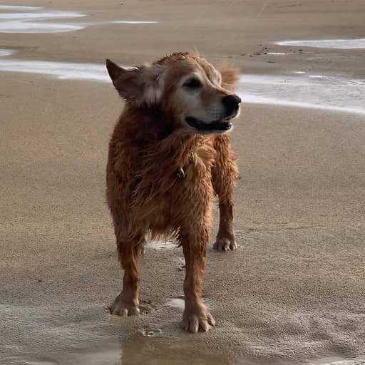
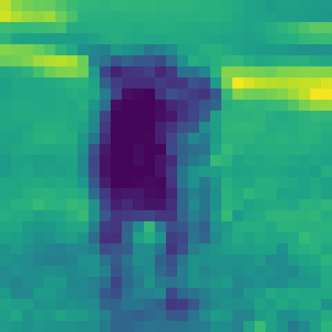
🔍 activations_conv2d

channel_6.png

Remember that at the beginning the convolution is looking at a very small part of the image, and as we go deeper into the network the convolutions take into account larger and larger windows of the original image. So the patterns they learn become more complex later on. The first layer of convolutions are really just learning to identify very simple shapes and patterns, akin to sensory processing.

In this case it looks like it's identifying the left side of dog. I'd recognise her anywhere.

channel_6.png

Oooo! Exciting! Nothing! This is a dead filter, which means that it never activated strongly on any of the training images. It's possible that if we trained for longer this filter might have learned something, but it's not looking likely.

In a layer down the line a "dead" layer like this might indicate that the CNN has formed a channel that only activates when a higher-level feature (like a horn, or a beak or a window) is present. So we'd understand if it didn't activate. But as it's all the start it's going to end up being a useless channel. Other neural-network architectures, like a Residual neural network, have ways of dealing with this problem, but we're not going to worry about it for now.

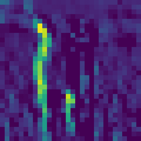
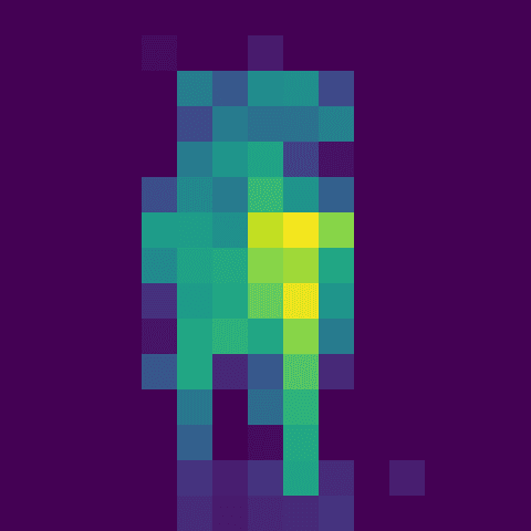
channel_26.png

In this image we can see the flat outline of the dog, and the rest of the image shows activations. This indicates this filter may have learned about a simple texture, and is activating when it sees that texture.

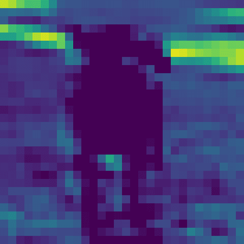
🔎 activations_conv2d_1

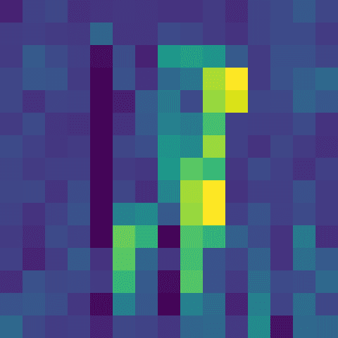
channel_9.png

Dog!

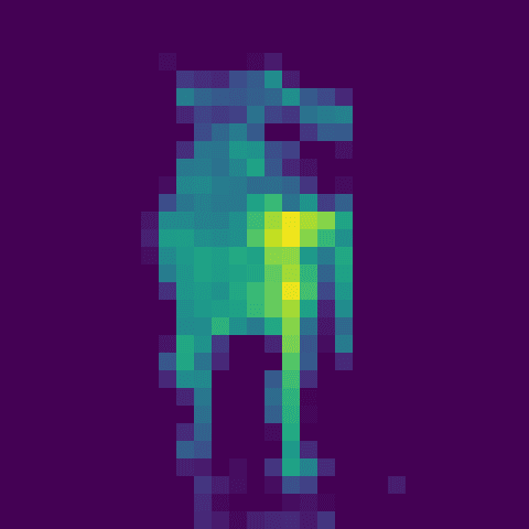
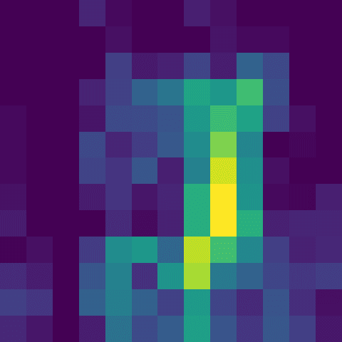
channel_13.png

This looks almost like a thermal camera. It could be that it's picking up the gradient the scene.

channel_25.png

Only a couple of bright pixels amid a blank output could mean a few things.

1. Bright spots mean strong activations, meaning the filter at this layer is highly responsive to specific features in the input image. It could be detecting shapes, textures, or patterns that are very pronounced in the input.
2. The features might be sparse. As there are a few activations, it suggests that the features being detected by this layer are sparse in the input. This isn't unusual, and might be picking up on more specific, less common features.
3. It could also be overfitting. In some cases, if these bright spots are too specific or too focused on certain pixels, it might indicate a tendency towards overfitting, where the model is learning to respond excessively to noise or very specific details in the training data.
4. This could also indicate that the filters in this layer are highly sensitive or perhaps too finely tuned to certain features.

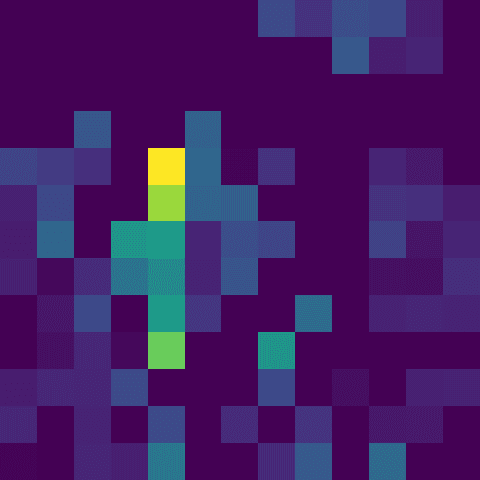
🕵 activations_conv2d_2

channel_9.png

channel_17.png

◼️ activations_dense

channel_12.png

channel_17.png

◾ activations_dense_1

channel_34.png

channel_59.png

?

We probably don't want to track all of these generated images, so let's add the output/ directory to our .gitignore file:

echo "output/" >> .gitignore

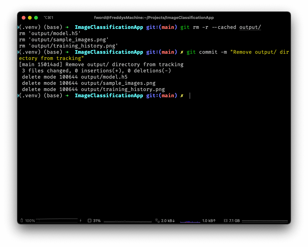
If we want to remove what's been tracked from that folder before, we can run:

git rm -r --cached output/

The commit these changes:

git commit -m "Remove output/ directory from tracking"

🏃 How to Run

Remember to activate the virtual environment, if you haven't already:

source .venv/bin/activate

Install any required packages:

pip install -r requirements.txt

If you haven't already, train a CNN:

python scripts/train.py

Then, to classify your own images run the following:

python scripts/classify.py <path/to/your/image.png>

And find the activation images in the output/ directory:

open output/

🗂️ Updated Files

Project structure

.
├── .venv/
├── .gitignore
├── resources
│   └── dog.jpg
├── output
│   ├── activations_conv2d/
│   ├── activations_conv2d_1/
│   ├── activations_conv2d_2/
│   ├── activations_dense/
│   ├── activations_dense_1/
│   ├── model.h5
│   ├── sample_images.png
│   └── training_history.png
├── scripts
│   ├── classify.py
│   └── train.py
├── README.md
└── requirements.txt

scripts/classify.py

from tensorflow.keras import models, preprocessing, Model
import sys
import os
import tensorflow as tf
import numpy as np
from matplotlib import pyplot as plt
from train import CLASS_NAMES  # Import class names for label mapping


def read_command_line_arguments():
    """
    Read the first command line argument as a image filepath.

    Returns:
        The image filepath.
    """
    if len(sys.argv) != 2:
        print(f"Requires exactly 1 input, but received {len(sys.argv) -1}")
        print(f"Use: python scripts/classify.py <path/to/image.png>")
        exit()
    input_image_filepath = sys.argv[1]
    return input_image_filepath


def load_image(path):
    """
    Load the image at the given filepath as an array of RGB component values

    Args:
        path: The path to the image to load.

    Returns:
        The image as an array of RGB component values.
    """

    # Load the image and resize it to match the model's expected input shape
    image = preprocessing.image.load_img(path, target_size=(32, 32))

    # Convert image to array
    image_array = preprocessing.image.img_to_array(image)

    # Expand dimensions for batch processing
    image_batch = tf.expand_dims(image_array, 0)

    # Normalise the image
    image_batch /= 255.0

    return image_batch


def visualise_intermediate_layers(model, image_batch, layer_names):
    """
    Visualise the activations of the intermediate layers of the model,
    saving images to the output/ directory.

    Args:
        model: The model to visualise.
        image_batch: The batch of images to use as input.
        layer_names: The names of the layers to visualise.
    """

    # Get the outputs of each layer in the model
    layer_outputs = [layer.output for layer in model.layers]
    # Create a new model for visualising the intermediate layers
    activation_model = Model(inputs=model.input, outputs=layer_outputs)
    # Get the layer activations
    activations = activation_model.predict(image_batch)

    # Loop through each layer and visualise its activations
    for layer_name, activation in zip(layer_names, activations):
        layer_dir = os.path.join("output", f"activations_{layer_name}")
        if not os.path.exists(layer_dir):
            os.makedirs(layer_dir)

        # Save each activation channel as an image
        num_channels = activation.shape[-1]
        for i in range(num_channels):
            plt.figure()
            plt.imshow(activation[0, :, :, i], cmap="viridis")
            plt.axis("off")
            plt.subplots_adjust(left=0, right=1, top=1, bottom=0)
            plt.savefig(os.path.join(
                layer_dir, f"channel_{i}.png"), bbox_inches="tight", pad_inches=0)
            plt.close()


if __name__ == "__main__":
    # Read image filepath from command line
    input_image_filepath = read_command_line_arguments()

    # Load and preprocess the image
    image_batch = load_image(input_image_filepath)

    # Load pre-trained model
    model = models.load_model(os.path.join("output", "model.h5"))

    # Perform image classification
    predictions = model.predict(image_batch)[0]
    predicted_class = np.argmax(predictions)
    print(f"Predicted class is: {CLASS_NAMES[predicted_class]}")

    # Print class probabilities
    for i in range(len(predictions)):
        class_name = CLASS_NAMES[i].ljust(16, " ")
        probability = "{:.1f}".format(predictions[i] * 100)
        print(f"{class_name} : {probability}%")

    # Visualise activations of intermediate layers
    layer_names = [
        layer.name for layer in model.layers if "conv" in layer.name or "dense" in layer.name]
    visualise_intermediate_layers(model, image_batch, layer_names)

.gitignore

# Byte-compiled / optimized / DLL files
__pycache__/
*.py[cod]
*$py.class

# C extensions
*.so

# Distribution / packaging
.Python
build/
develop-eggs/
dist/
downloads/
eggs/
.eggs/
lib/
lib64/
parts/
sdist/
var/
wheels/
share/python-wheels/
*.egg-info/
.installed.cfg
*.egg
MANIFEST

# PyInstaller
#  Usually these files are written by a python script from a template
#  before PyInstaller builds the exe, so as to inject date/other infos into it.
*.manifest
*.spec

# Installer logs
pip-log.txt
pip-delete-this-directory.txt

# Unit test / coverage reports
htmlcov/
.tox/
.nox/
.coverage
.coverage.*
.cache
nosetests.xml
coverage.xml
*.cover
*.py,cover
.hypothesis/
.pytest_cache/
cover/

# Translations
*.mo
*.pot

# Django stuff:
*.log
local_settings.py
db.sqlite3
db.sqlite3-journal

# Flask stuff:
instance/
.webassets-cache

# Scrapy stuff:
.scrapy

# Sphinx documentation
docs/_build/

# PyBuilder
.pybuilder/
target/

# Jupyter Notebook
.ipynb_checkpoints

# IPython
profile_default/
ipython_config.py

# pyenv
#   For a library or package, you might want to ignore these files since the code is
#   intended to run in multiple environments; otherwise, check them in:
# .python-version

# pipenv
#   According to pypa/pipenv#598, it is recommended to include Pipfile.lock in version control.
#   However, in case of collaboration, if having platform-specific dependencies or dependencies
#   having no cross-platform support, pipenv may install dependencies that don't work, or not
#   install all needed dependencies.
#Pipfile.lock

# poetry
#   Similar to Pipfile.lock, it is generally recommended to include poetry.lock in version control.
#   This is especially recommended for binary packages to ensure reproducibility, and is more
#   commonly ignored for libraries.
#   https://python-poetry.org/docs/basic-usage/#commit-your-poetrylock-file-to-version-control
#poetry.lock

# pdm
#   Similar to Pipfile.lock, it is generally recommended to include pdm.lock in version control.
#pdm.lock
#   pdm stores project-wide configurations in .pdm.toml, but it is recommended to not include it
#   in version control.
#   https://pdm.fming.dev/#use-with-ide
.pdm.toml

# PEP 582; used by e.g. github.com/David-OConnor/pyflow and github.com/pdm-project/pdm
__pypackages__/

# Celery stuff
celerybeat-schedule
celerybeat.pid

# SageMath parsed files
*.sage.py

# Environments
.env
.venv
env/
venv/
ENV/
env.bak/
venv.bak/

# Spyder project settings
.spyderproject
.spyproject

# Rope project settings
.ropeproject

# mkdocs documentation
/site

# mypy
.mypy_cache/
.dmypy.json
dmypy.json

# Pyre type checker
.pyre/

# pytype static type analyzer
.pytype/

# Cython debug symbols
cython_debug/

# PyCharm
#  JetBrains specific template is maintained in a separate JetBrains.gitignore that can
#  be found at https://github.com/github/gitignore/blob/main/Global/JetBrains.gitignore
#  and can be added to the global gitignore or merged into this file.  For a more nuclear
#  option (not recommended) you can uncomment the following to ignore the entire idea folder.
#.idea/

/output