2. Training a convolutional neural network

In the last lesson we created a GitHub repository, and set up our project ready to run Python code. In this lesson we're going to put that to good use training a machine learning model!

A Convolutional Neural Network (CNN) is a type of deep learning model that works well in image recognition and processing tasks.

CNNs are especially good at capturing spatial hierarchies of features. They work by applying a series of filters (kernels) to local regions of the input. The same filter is applied across the image, learning features irrespective of their position.

Early layers capture small parts of the input, like edges and textures. And as layers progress, they combine simpler features to form higher-level abstractions. Deep layers integrate features from earlier ones, capturing complex shapes and objects.

This hierarchical approach is naturally suited for tasks like image recognition, where the spatial relationship between pixels is crucial.

We're going to use tensorflow to train our CNN, and we're going to use matplotlib to show us the training data.

Open up requirements.txt and add the new dependancy:

tensorflow
matplotlib

Install the listed dependencies using:

pip install -r requirements.txt

Rename the test.py file to train.py, and then replace its contents with this script:

from tensorflow.keras import models, layers, datasets
from matplotlib import pyplot as plt
import random
import os
import tensorflow as tf

if __name__ == "__main__":
    # Create output directory
    if not os.path.exists("output"):
        os.mkdir("output")

    # Load CIFAR-10 data
    (train_images, train_labels), (test_images, test_labels) = datasets.cifar10.load_data()

    # Plot sample images
    plot_images(train_images, train_labels)

    # Normalize images
    train_images, test_images = train_images / 255.0, test_images / 255.0

    # Model creation and summary
    model = create_model()
    model.summary()

    # Model compilation and training
    model.compile(optimizer='adam',
                  loss=tf.keras.losses.SparseCategoricalCrossentropy(from_logits=False),
                  metrics=['accuracy'])
    history = model.fit(train_images, train_labels, epochs=10,
                        validation_data=(test_images, test_labels))

    # Plot training history
    plot_training_history(history)

    # Model evaluation
    test_loss, test_acc = model.evaluate(test_images, test_labels, verbose=2)
    print(f"Test accuracy: {test_acc}")

    # Save the model
    model.save(os.path.join("output", "model.h5"))

This script will:

1. Import our dependancies
2. If this is the "main" script, execute the following lines:
3. Create an output directory, if it does not already exist
4. Load the CIFAR-10 dataset images
5. Plot those images, along with their respective labels
6. Normalise the images so that RGB channel values range from 0.0 to 1.0
7. Define our machine learning model
8. Train this model on the dataset
9. Plot the training history out to a file
10. Print an estimate of the model accuracy
11. Save the model to an output file, so that we can load it back in the future

and now we need to define some of those functions!

🖼️ CIFAR-10

Note how we're using the CIFAR-10 dataset, which was developed by the Canadian Institute for Advanced Research (CIFAR).

CIFAR-10 is a labeled dataset for image classification. It has 60,000 32x32 color images, divided into 10 classes like 'airplane', 'cat', etc.

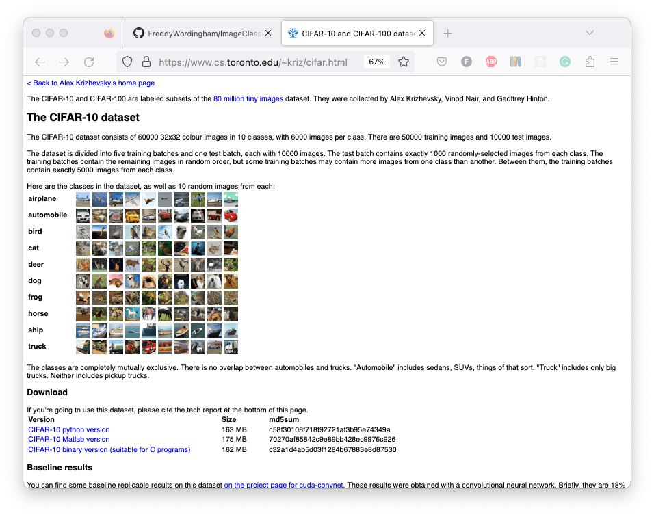
The training set comprises 50,000 images, and the test set has 10,000. It's commonly used for machine learning models like CNNs.

Each class has 6,000 images, but it's only a subset of the 80-million tiny images dataset.

Collecting and labeling a custom dataset can be very labor-intensive. Using CIFAR-10 saves time and effort. It's a well-vetted, diverse dataset ideal for initial testing and prototyping. Benchmarking against it helps compare your models to existing solutions.

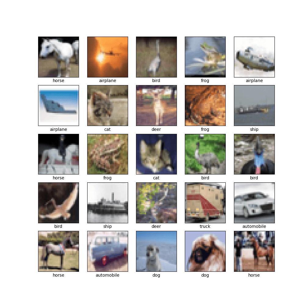
📸 Plot Images

# Constants for class names
CLASS_NAMES = [
    "airplane", "automobile", "bird", "cat", "deer",
    "dog", "frog", "horse", "ship", "truck"
]


def plot_images(train_images, train_labels):
    """
    Plot a random selection of images with their labels.

    Args:
        train_images: The images to plot.
        train_labels: The respective numerical class labels for the images.
    """

    # Create a new square figure
    plt.figure(figsize=(10, 10))

    # Plot 25 random images
    for i in range(25):
        n = random.randint(0, len(train_images))
        plt.subplot(5, 5, i + 1)
        plt.xticks([])
        plt.yticks([])
        plt.grid(False)
        plt.imshow(train_images[n])
        plt.xlabel(CLASS_NAMES[train_labels[n][0]])

    # Save the figure
    plt.savefig(os.path.join("output", "sample_images.png"))

This function uses matplotlib to plot 25 random images from the train_images dataset. Labels from train_labels are displayed under each image.

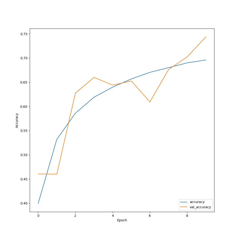
📈 Plot Training History

def plot_training_history(history):
    """
    Plot training and validation accuracy over epochs.

    Args:
        history: The training history of the model.
    """

    plt.figure(figsize=(10, 10))
    plt.plot(history.history["accuracy"], label="accuracy")
    plt.plot(history.history["val_accuracy"], label="val_accuracy")
    plt.xlabel("Epoch")
    plt.ylabel("Accuracy")
    plt.legend(loc="lower right")
    plt.savefig(os.path.join("output", "training_history.png"))

This function plots the accuracy as it increases with training epochs.

📐 Define the Model

def create_model():
    """
    Create a convolutional neural network model for image classification.

    Returns:
        The CNN model.
    """

    model = models.Sequential()

    # Convolutional layers
    model.add(layers.Conv2D(
        32, (3, 3), activation='relu', input_shape=(32, 32, 3)))
    model.add(layers.BatchNormalization())
    model.add(layers.MaxPooling2D((2, 2)))
    model.add(layers.Dropout(0.25))

    model.add(layers.Conv2D(64, (3, 3), activation='relu'))
    model.add(layers.BatchNormalization())
    model.add(layers.MaxPooling2D((2, 2)))
    model.add(layers.Dropout(0.25))

    model.add(layers.Conv2D(128, (3, 3), activation='relu'))
    model.add(layers.BatchNormalization())
    model.add(layers.MaxPooling2D((2, 2)))
    model.add(layers.Dropout(0.25))

    # Flattening for dense layers
    model.add(layers.Flatten())

    # Dense layers
    model.add(layers.Dense(128, activation='relu'))
    model.add(layers.BatchNormalization())
    model.add(layers.Dropout(0.5))
    model.add(layers.Dense(10, activation='softmax'))

    return model

This function defines the architecture of our model:

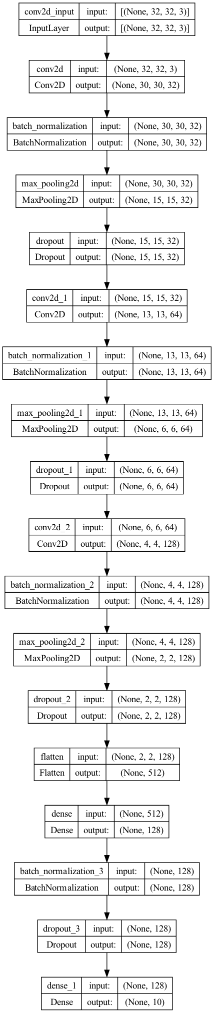
We use three sets of convolutional layers, each followed by batch normalisation, max pooling, and a dropout layer. This helps the model extract hierarchical features from the image and prevents overfitting. After the convolutional layers, we flatten the output to feed it into two dense layers. The final dense layer uses a softmax activation function to produce a probability distribution over 10 classes.

• Convolutional layers are for feature extraction.
• Batch normalisation helps in faster and more stable training.
• MaxPooling reduces the dimensionality.
• Dropout helps in preventing overfitting.
• Dense layers are for classification.
• Softmax is used for multi-class classification.

Now running this script will start a model training on the CIFAR-10 data:

python scripts/train.py

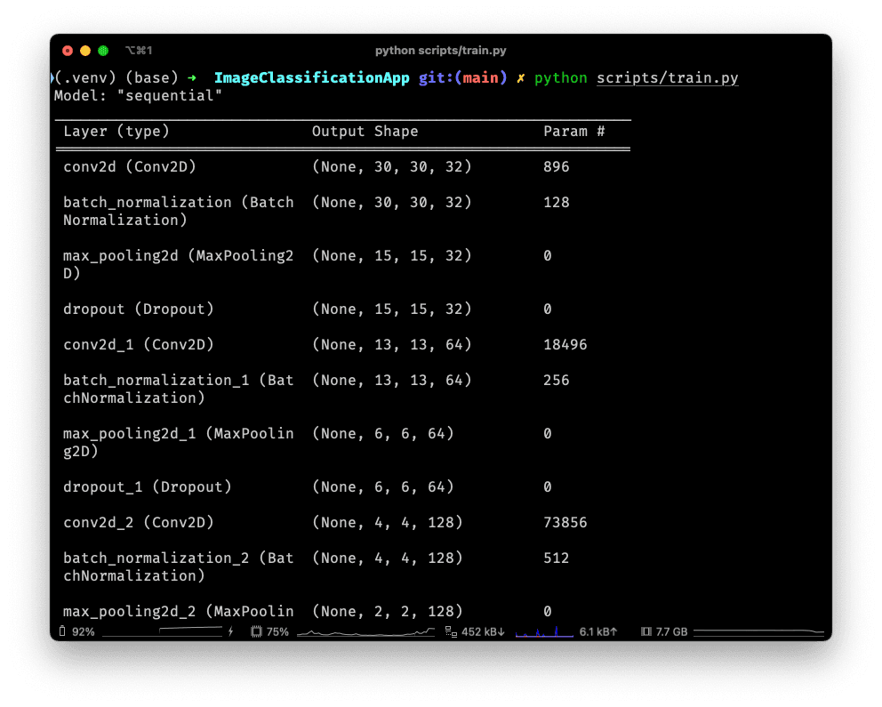
After it completes 10 epochs it will save the model progress to output/model.h5

🏃‍♀ How to Run

Set the working directory to the root of the project, and activate the virtual environment:

source .venv/bin/activate

Install the new required packages:

pip install -r requirements.txt

Train a CNN, and save it to output/model.h5:

python scripts/train.py

🔮 CNN Layers and Terms

Conv2D: Convolutional layers are the major building blocks of CNNs. They understand the local patterns of the image and extract features like edges, corners and textures from the input images. By using kernels (functions which scan over the image), it will create feature maps that summarise the presence of those features in the input.

BatchNormalization: Normalise the activations of the neurons so that the mean activation is close to 0 and the activation standard deviation is close to 1. This helps in faster training and prevents the problem of vanishing gradients.

MaxPooling2D: Reduces the dimensionality of each feature map but retains the most important information. It also helps in reducing the computational complexity of the model.

Dropout: Randomly drops a fraction of neurons during training. This helps in preventing overfitting.

Flatten: Converts the 2D feature maps to a 1D feature vector. This is required to connect the CNN to a fully connected layer.

Dense: Fully connected layers are the traditional neural networks that are used for classification and regression. They connect every neuron in one layer to every neuron in another layer. The "Universal Approximation Theorem" states that a neural network with a single hidden layer can approximate any continuous function to arbitrary accuracy. This is why fully connected layers are so powerful.

ReLU: Rectified Linear Unit is a non-linear activation function. It helps in introducing non-linearity to the model. Without it, the model would be just a linear regression model, which is not very powerful.

Softmax: Converts the output to a probability distribution. Each element in the output vector represents the probability of a particular class. The sum of all the elements in the output vector is 1.

Adam Optimiser: Adaptive Moment Estimation (Adam) is an optimisation algorithm used to minimise the loss function during training. It combines the benefits of two other extensions of stochastic gradient descent: AdaGrad and RMSProp.

📚 Further Reading

1. Convolutional Neural Networks (CNNs) Explained
2. Understanding Max Pooling in Deep Learning
3. How Dropout Prevents Overfitting
4. Gentle Introduction to the Adam Optimization Algorithm for Deep Learning

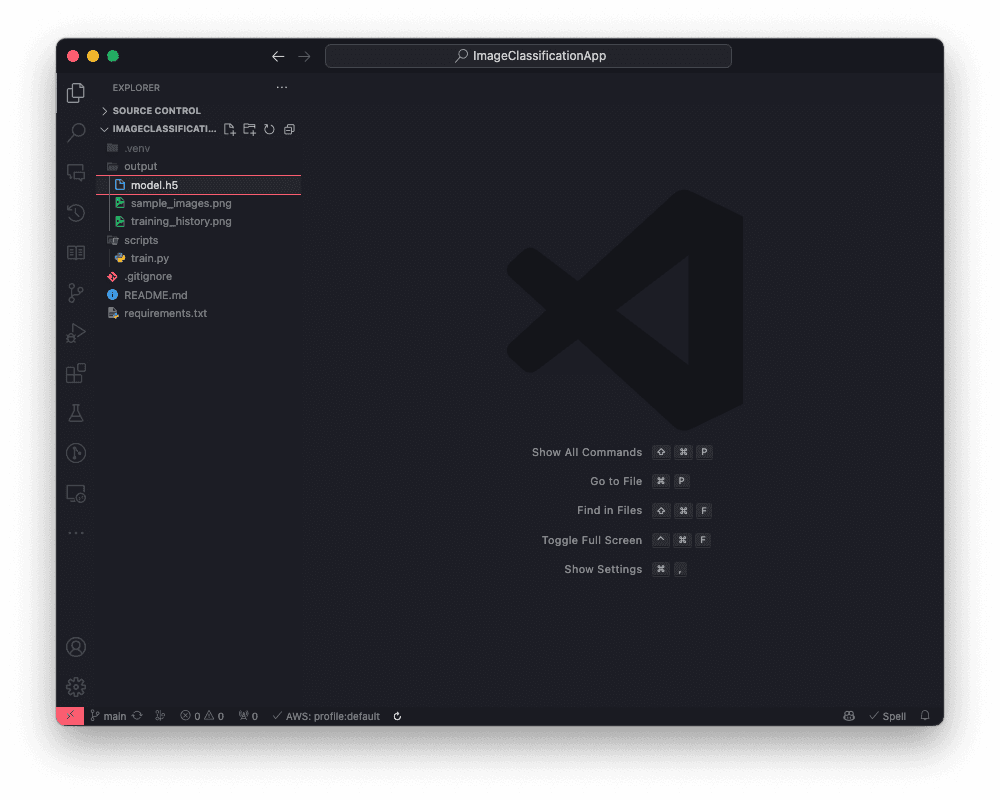
🗂️ Updated Files

Project structure

.
├── .venv/
├── .gitignore
├── output
│   ├── model.h5
│   ├── sample_images.png
│   └── training_history.png
├── scripts
│   └── train.py
├── README.md
└── requirements.txt

requirements.txt

tensorflow
matplotlib

scripts/train.py

from tensorflow.keras import models, layers, datasets
from matplotlib import pyplot as plt
import random
import os
import tensorflow as tf

# Constants for class names
CLASS_NAMES = [
    "airplane", "automobile", "bird", "cat", "deer",
    "dog", "frog", "horse", "ship", "truck"
]


def plot_images(train_images, train_labels):
    """
    Plot a random selection of images with their labels.

    Args:
        train_images: The images to plot.
        train_labels: The respective numerical class labels for the images.
    """

    # Create a new square figure
    plt.figure(figsize=(10, 10))

    # Plot 25 random images
    for i in range(25):
        n = random.randint(0, len(train_images))
        plt.subplot(5, 5, i + 1)
        plt.xticks([])
        plt.yticks([])
        plt.grid(False)
        plt.imshow(train_images[n])
        plt.xlabel(CLASS_NAMES[train_labels[n][0]])

    # Save the figure
    plt.savefig(os.path.join("output", "sample_images.png"))


def plot_training_history(history):
    """
    Plot training and validation accuracy over epochs.

    Args:
        history: The training history of the model.
    """

    plt.figure(figsize=(10, 10))
    plt.plot(history.history["accuracy"], label="accuracy")
    plt.plot(history.history["val_accuracy"], label="val_accuracy")
    plt.xlabel("Epoch")
    plt.ylabel("Accuracy")
    plt.legend(loc="lower right")
    plt.savefig(os.path.join("output", "training_history.png"))


def create_model():
    """
    Create a convolutional neural network model for image classification.

    Returns:
        The CNN model.
    """

    model = models.Sequential()

    # Convolutional layers
    model.add(layers.Conv2D(
        32, (3, 3), activation='relu', input_shape=(32, 32, 3)))
    model.add(layers.BatchNormalization())
    model.add(layers.MaxPooling2D((2, 2)))
    model.add(layers.Dropout(0.25))

    model.add(layers.Conv2D(64, (3, 3), activation='relu'))
    model.add(layers.BatchNormalization())
    model.add(layers.MaxPooling2D((2, 2)))
    model.add(layers.Dropout(0.25))

    model.add(layers.Conv2D(128, (3, 3), activation='relu'))
    model.add(layers.BatchNormalization())
    model.add(layers.MaxPooling2D((2, 2)))
    model.add(layers.Dropout(0.25))

    # Flattening for dense layers
    model.add(layers.Flatten())

    # Dense layers
    model.add(layers.Dense(128, activation='relu'))
    model.add(layers.BatchNormalization())
    model.add(layers.Dropout(0.5))
    model.add(layers.Dense(10, activation='softmax'))

    return model


if __name__ == "__main__":
    # Create output directory
    if not os.path.exists("output"):
        os.mkdir("output")

    # Load CIFAR-10 data
    (train_images, train_labels), (test_images,
                                   test_labels) = datasets.cifar10.load_data()

    # Plot sample images
    plot_images(train_images, train_labels)

    # Normalize images
    train_images, test_images = train_images / 255.0, test_images / 255.0

    # Model creation and summary
    model = create_model()
    model.summary()

    # Model compilation and training
    model.compile(optimizer='adam',
                  loss=tf.keras.losses.SparseCategoricalCrossentropy(
                      from_logits=False),
                  metrics=['accuracy'])
    history = model.fit(train_images, train_labels, epochs=10,
                        validation_data=(test_images, test_labels))

    # Plot training history
    plot_training_history(history)

    # Model evaluation
    test_loss, test_acc = model.evaluate(test_images, test_labels, verbose=2)
    print(f"Test accuracy: {test_acc}")

    # Save the model
    model.save(os.path.join("output", "model.h5"))

plot_images: Randomly picks 25 images from the training set and plots them in a 5x5 grid. It's useful for checking the data.

plot_training_history: Plots the training and validation accuracy across epochs. Helps in understanding how well the model is learning.

create_model: Defines the CNN architecture. It has three Conv2D layers with different numbers of filters, followed by BatchNormalisation, MaxPooling, and Dropout. After the Conv layers, there's a Flatten layer to prepare the data for the Dense layers.

Main Code: Checks and creates an output directory for storing plots and models. Loads CIFAR-10 data for the training and test set. Normalises the images by dividing by 255. This is a common preprocessing step. Summarises the model architecture before training. Compiles and trains the model, saving the history for plotting.